Homework 5 - The eternal significance of publications and citations!

Citation networks, intricately woven through references in scholarly papers, play a pivotal role in mapping the evolution of knowledge in academic research. Analyzing these networks is essential for identifying influential works, tracking idea development, and gauging the impact of research. Leveraging graph analysis enhances our ability to uncover hidden patterns, predict emerging trends, and comprehend the intricate relationships within these networks.

This time, you and your team have decided to dive deep into the citation realm. Now, you will deal with graphs to determine relevant characteristics and highlights from the relations among those publications.

Let's hands-on this!

In this Homework, you will explore the paper citation universe, exploring relations among multiple academic publications!

• Backend: where you need to develop efficient algorithms that define the functionalities of the system
• Frontend: where you provide visualization for queries entered by the user

IMPORTANT: To deal with functionalities 1 and 2 and visualization of graphs, you can freely use libraries such as networkx or any other tool you choose. Still, when writing an algorithm for functionalities 3, 4, and 5, it must be implemented yourself using proper data structures, without any library that computes some algorithm steps for you.

---

1. Data

In this homework, you will work on a dataset that contains information about a group of papers and their citation relationships. You can find and download the dataset here

Graphs setup

Based on the available data, you will create two graphs to model our relationships as follows:

1. Citation graph: This graph should represent the paper's citation relationships. We want this graph to be unweighted and directed. The citation should represent the citation given from one paper to another. For example, if paper A has cited paper B, we should expect an edge from node A to B.

2. Collaboration graph: This graph should represent the collaborations of the paper's authors. This graph should be weighted and undirected. Consider an appropriate weighting scheme for your edges to make your graph weighted.

Data pre-processing

The dataset is quite large and may not fit in your memory when you try constructing your graph. So, what is the solution? You should focus your investigation on a subgraph. You can work on the most connected component in the graph. However, you must first construct and analyze the connections to identify the connected components.

As a result, you will attempt to approximate that most connected component by performing the following steps:

1. Identify the top 10,000 papers with the highest number of citations.

2. Then the nodes of your graphs would be as follows:

   Citation graph: you can consider each of the papers as your nodes

   Collaboration graph: the authors of these papers would be your nodes

3. For the edges of the two graphs, you would have the following cases:

   Citation graph: only consider the citation relationship between these 10,000 papers and ignore the rest.

   Collaboration graph: only consider the collaborations between the authors of these 10,000 papers and ignore the rest.

---

Here's several helpful packages to load and set-up

import numpy as np
import pandas as pd
import ijson
import time
import csv
import numpy as np
from decimal import Decimal
import matplotlib as mpl
import matplotlib.pyplot as plt
import networkx as nx
from itables import init_notebook_mode
from libs.backend import * # Custom backend functionalities
from libs.frontend import * # Custom frontend to display backend functionalities
import ipywidgets as widgets
import warnings

# Make sure that plots are in-line
%matplotlib inline
# Make the tables interactive
init_notebook_mode(all_interactive=True)
# Set plot grid parameter
mpl.rcParams['grid.linestyle'] = "-" 
# Suppress DeprecationWarnings from IpyWidgets
warnings.filterwarnings('ignore')

Converting Json to CSV (https://www.kaggle.com/code/shreyasbhatk/csv-conversion-all-fields)

start = time.process_time()

PAPER = []
Author = []
count = 0

with open('dblp.v12.json', "rb") as f, open("output.csv", "w", newline="") as csvfile:
    fieldnames = ['id', 'title', 'year', 'author_name', 'author_org', 'author_id', 'n_citation', 'doc_type',
                  'reference_count', 'references', 'venue_id', 'venue_name', 'venue_type', 'doi', 'keyword','volume','issue','publisher',
                  'weight', 'indexed_keyword', 'inverted_index']
    writer = csv.DictWriter(csvfile, fieldnames=fieldnames)
    writer.writeheader()

    for i, element in enumerate(ijson.items(f, "item")):
        paper = {}
        paper['id'] = element['id']
        paper['title'] = element['title']

        year = element.get('year')
        if year:
            paper['year'] = year
        else:
            paper['year'] = np.nan

        author = element.get('authors')
        if author:
            Author = element['authors']
            author_name = []
            author_org = []
            author_id = []

            for i in Author:
                if 'name' in i and 'id' in i and 'org' in i:
                    author_name.append(str(i['name']))  # Convert to string
                    author_id.append(str(i['id']))
                    author_org.append(str(i['org']))
                else:
                    author_name.append(str(np.nan))  # Convert to string
                    author_id.append(str(np.nan))
                    author_org.append(str(np.nan))

            paper['author_name'] = ';'.join(author_name)
            paper['author_org'] = ';'.join(author_org)
            paper['author_id'] = ';'.join(author_id)

        n_citation = element.get('n_citation')
        if n_citation:
            paper['n_citation'] = n_citation
        else:
            paper['n_citation'] = np.nan

        doc_type = element.get('doc_type')
        if doc_type:
            paper['doc_type'] = doc_type
        else:
            paper['doc_type'] = np.nan

        references = element.get('references')
        if references:
            paper['reference_count'] = len(references)
            paper['references'] = ';'.join(str(int(r)) for r in references)
        else:
            paper['references'] = np.nan

        venue = element.get('venue')
        if venue:
            if 'id' in venue and 'raw' in venue and 'type' in venue:
                paper['venue_id'] = str(venue['id'])
                paper['venue_name'] = venue['raw']
                paper['venue_type'] = venue['type']
            else:
                paper['venue_id'] = np.nan
                paper['venue_name'] = np.nan
                paper['venue_type'] = np.nan
        else:
            paper['venue_id'] = np.nan
            paper['venue_name'] = np.nan
            paper['venue_type'] = np.nan

        doi = element.get('doi')
        if doi:
            paper['doi'] = f"https://doi.org/{doi}"
        else:
            paper['doi'] = np.nan

        fos = element.get('fos')
        if fos:
            fosunparsed = element['fos']
            keyword = []
            weight = []

            for i in fosunparsed:
                if isinstance(i['w'], (int, float, Decimal)):
                    keyword.append(str(i['name']))  # Convert to string
                    weight.append(str(i['w']))
                else:
                    keyword.append(str(np.nan))  # Convert to string
                    weight.append(str(np.nan))

        else:
            keyword = []
            weight = []

        paper['keyword'] = ';'.join(keyword)
        paper['weight'] = ';'.join(weight)

        indexed_abstract = element.get('indexed_abstract')
        if indexed_abstract:
            indexed_abstracts = indexed_abstract.get('InvertedIndex')
            inverted_vector = []
            keywords = []

            for i in indexed_abstracts:
                if i:
                    keywords.append(str(i))  # Convert to string
                    inverted_vector.append(str(indexed_abstracts[i]))  # Convert to string
        else:
            keywords = []
            inverted_vector = []

        paper['indexed_keyword'] = ';'.join(keywords)
        paper['inverted_index'] = ';'.join(inverted_vector)
        
        publisher= element.get('publisher')
        if publisher:
            paper['publisher']=publisher
        else:
            paper['publisher']=np.nan
        volume = element.get('volume')
        if volume:
            paper['volume']=volume
        else:
            paper['volume']=np.nan
        issue = element.get('issue')
        if issue:
            paper['issue']=issue
        else:
            paper['issue']=np.nan
        count += 1
        writer.writerow(paper)

        if count % 4800 == 0:
            print(f"{count}:{round((time.process_time() - start), 2)}s ", end="")

---

Data Pre-processing Algorithm

Step 1: Load Data and Identify Top 10,000 Papers

1. Load the dataset into a Pandas DataFrame.
2. Sort the DataFrame by the n_citation column in descending order to get the papers with the highest number of citations.
3. Slice the top 10,000 records to work with.

Step 2: Construct Nodes for Both Graphs

• For the Citation Graph:
  • Extract the id field of the top 10,000 papers to use as nodes.
• For the Collaboration Graph:
  • Extract the author_id fields of the top 10,000 papers, parse the individual author IDs, and use them as nodes.

Step 3: Construct Edges for Both Graphs

• For the Citation Graph:
  • For each of the top 10,000 papers, parse its references field to find other papers it cites.
  • Filter those references to only include papers within the top 10,000.
  • Add directed edges from the citing paper to the cited papers.
• For the Collaboration Graph:
  • For each paper, parse the author_id field to find all pairs of authors that have collaborated.
  • Add undirected edges between these authors.
  • The weighting scheme could be the number of papers co-authored by the pair, meaning each additional paper they co-author together increases the weight of the edge by one.

Approximating the Most Connected Component

To identify the most connected component, we would analyze the constructed graphs:

1. Use NetworkX to find connected components in the collaboration graph (since it's undirected) and weakly connected components in the citation graph (since it's directed).
2. Determine the size of each component.
3. Identify the largest component.

Code Implementation:

# Load data into a Pandas DataFrame
df = pd.read_csv('output.csv')

# Sort by number of citations and get the top 10,000 papers
top_papers = df.sort_values('n_citation', ascending=False).head(10000)

# Citation Graph Nodes
citation_nodes = top_papers['id'].tolist()

# Collaboration Graph Nodes
collaboration_nodes = set()

# Before applying the lambda, ensure NaN values are handled, e.g., by converting to a string
top_papers['author_id'] = top_papers['author_id'].fillna('')

# Now applying the lambda function
top_papers['author_id'].str.split(';').apply(lambda x: collaboration_nodes.update(x) if isinstance(x, list) else None)
# Empty and NaN ids are dropped
collaboration_nodes.remove('')
collaboration_nodes.remove('nan')

# Create graphs
citation_graph = nx.DiGraph()
collaboration_graph = nx.Graph()

# Add nodes to graphs
citation_graph.add_nodes_from(citation_nodes)
collaboration_graph.add_nodes_from(collaboration_nodes)

# Create a dictionary with authors ids as keys and authors names as values
authors_names = dict()
top_papers.apply(lambda row: authors_names.update(dict(zip(row['author_id'].split(';'),row['author_name'].split(';')))) if not(pd.isna(row['author_name'])) else None, axis = 1)
# NaN name is dropped
del authors_names['nan']

# Add papers titles and authors names to node attributes
nx.set_node_attributes(citation_graph, dict(zip(top_papers.id, top_papers.title)), name = 'title')
nx.set_node_attributes(collaboration_graph, authors_names, name = 'author_name')

# Add edges to Citation Graph
for _, row in top_papers.iterrows():
    if pd.notna(row['references']):
        cited_papers = [int(x) for x in row['references'].split(';') if x.isdigit()]
        for cited in cited_papers:
            if cited in citation_nodes:
                citation_graph.add_edge(row['id'], cited)

# Add edges to Collaboration Graph with a simple weighting scheme
edges_labels = dict()
for _, row in top_papers.iterrows():
    authors = str(row['author_id']).split(';') if pd.notnull(row['author_id']) else []
    authors = [obj for obj in authors if obj != 'nan']
    for i, author_i in enumerate(authors):
        for author_j in authors[i+1:]:
            if author_i and author_j:  # Ensure author_i and author_j are not empty strings
                if collaboration_graph.has_edge(author_i, author_j):
                    collaboration_graph[author_i][author_j]['weight'] += 1
                else:
                    collaboration_graph.add_edge(author_i, author_j, weight=1)
                    edges_labels.update({(author_i,author_j):row['title']})

# Associate to each edge of the collaboration graph the name of the correspondent paper
nx.set_edge_attributes(collaboration_graph, edges_labels, name = 'paper')

# Identify the largest connected component in the collaboration graph
largest_collaboration_cc = max(nx.connected_components(collaboration_graph), key=len)
subgraph_collaboration_graph = collaboration_graph.subgraph(largest_collaboration_cc)

# Visualizing the citation graph
plt.figure(figsize=(12, 8))
pos = nx.spring_layout(citation_graph)
nx.draw(citation_graph, pos, node_size=10, arrows=True, edge_color='red', with_labels=False)
plt.title("Citation Graph")
plt.show()

# Visualizing the collaboration graph
plt.figure(figsize=(12, 8))
pos = nx.spring_layout(collaboration_graph)
nx.draw(collaboration_graph, pos, node_size=10, edge_color='gray', with_labels=False)
plt.title("Collaboration Graph")
plt.show()

Visualizing the Largest Connected Component in the Collaboration Graph

# Visualizing the Largest Connected Component in the Collaboration Graph
plt.figure(figsize=(12, 8))
pos = nx.spring_layout(subgraph_collaboration_graph)
nx.draw(subgraph_collaboration_graph, pos, node_size=10, edge_color='gray', with_labels=False)
plt.title("Largest Connected Component in the Collaboration Graph")
plt.show()

---

To save or export the graphs as GraphML

# Assuming citation_graph and collaboration_graph are already created NetworkX graph objects
nx.write_graphml(citation_graph, "citation_graph.graphml")
nx.write_graphml(collaboration_graph, "collaboration_graph.graphml")
nx.write_graphml(subgraph_collaboration_graph, "subgraph_collaboration_graph.graphml")

To read or import the saved graphs from GraphML

citation_path = 'citation_graph.graphml'
collaboration_path = 'collaboration_graph.graphml'
subcollaboration_path = 'subgraph_collaboration_graph.graphml'

# Load the citation graph from GraphML file
citation_graph = nx.read_graphml(citation_path)

# Load the collaboration graph from GraphML file
collaboration_graph = nx.read_graphml(collaboration_path)

# Load the subgraph collaboration graph from GraphML file
subgraph_collaboration_graph = nx.read_graphml(subcollaboration_path)

---

2. Controlling system

In this section, five different functionalities to analyze the produced graphs are implemented from scratch and their outputs are visualized. You can check the full code inside the files backend.py (implementation) and frontend.py (visualization).
Please note that the visualizations are interactive, making the user able to dinamically select the functionalities' arguments. Unfortunately, only the static outputs are displayed if you're reviewing this notebook at the link https://ambarchatterjee.github.io/ADM_HW5_Group21. The widgets are trurly interactive if and only if the notebook is run in local.

Functionality 1 - Graph's features

This first functionality permits to examine a graph and report some of its features. Leveraging the library networkX, it takes in input the graph and (eventually) an integer k, returning the following items:

• A table containing the following general information about the graph:
  • Number of nodes in the graph
  • Number of the edges in the graph
  • Density of the graph
  • Average degree of the graph
  • Whether the network is sparse or dense
• A table that lists the graph's hubs
• A plot depicting the distribution of the citations received by papers (Citation graph)
• A plot depicting the distribution of the given citations by papers (Citation graph)
• A plot depicting the number of collaborations of the top k authors by degree (Collaboration graph)

To have a better understanding of the data, it was executed on both the Citation and Collaboration Graphs.

# CITATION GRAPH
first_funct = widgets.interactive(visual_1, 
                          {'manual': True},
                          G = widgets.Dropdown(options=[('Citation Graph',citation_graph),('Collaboration Graph',collaboration_graph),('Collaboration Graph (Largest Component)',subgraph_collaboration_graph)], description='Graph:'),
                          k = widgets.IntSlider(min = 2, max = 50, step = 1, value = 20, description = 'Top Authors:'))
first_funct.children[-1].layout.height = '1450px'
display(first_funct)

# COLLABORATION GRAPH
first_funct = widgets.interactive(visual_1, 
                          {'manual': True},
                          G = widgets.Dropdown(options=[('Citation Graph',citation_graph),('Collaboration Graph',collaboration_graph),('Collaboration Graph (Largest Component)',subgraph_collaboration_graph)], description='Graph:'),
                          k = widgets.IntSlider(min = 2, max = 50, step = 1, value = 20, description = 'Top Authors:'))
first_funct.children[-1].layout.height = '1450px'
display(first_funct)

From the tables we deduct that both the graphs are very sparse, with a density near to zero.
The average degree reflects this state: taking a look at the hubs, it can be deducted that there are a lot of nodes with a low degree (the 95th percentile is 30 for the Citation Graph and 24 for the Collaboration Graph, which are very low numbers considering that there are at least 10,000 node for each graph). The given and received citations distributions (Citation Graph) are almost equal, with a frequency peak in the first class: this is another confirm of what was asserted before about the sparseness of the graphs. The author who collaborated the most is: Rodrigo Lopez

Functionality 2 - Nodes' contribution

This functionality uses the methods embedded in the networkX library to compute the following centrality measures for a chosen node:

• Betweeness Centrality: measures the number of times a node lies on the shortest path between other nodes.
• PageRank: It's a variant of EigenCentrality which takes account for link direction. EigenCentrality takes account of the degree of nodes connected to the original node and so on.
• Closeness Centrality: it's the reciprocal of the sum of the length of the shortest path between the node and each other node.
• Degree Centrality: it's the normalized degree of the node (its degree divided by the maximum possible degree).

The results are displayed in a table. Please note that, since it is needed to specify the node id to calculate the centrality measures, a node id finder was added: it makes the user able to find a node id by typing either the author's name or the paper's title.

finder = widgets.interactive(visual_id_finder, 
                          {'manual': True},
                          G = widgets.Dropdown(options=[('Citation Graph',citation_graph),('Collaboration Graph',collaboration_graph),('Collaboration Graph (Largest Component)',subgraph_collaboration_graph)], description='Graph:'),
                          input_str = widgets.Text(value='',placeholder='Type name or title',description='Name/Title:'))
finder.children[-1].layout.height = '200px'
display(finder)

second_funct = widgets.interactive(visual_2, 
                          {'manual': True},
                          G = widgets.Dropdown(options=[('Citation Graph',citation_graph),('Collaboration Graph',collaboration_graph),('Collaboration Graph (Largest Component)',subgraph_collaboration_graph)], description='Graph:'),
                          v = widgets.Text(value='',placeholder='Type node ID',description='Node ID:'))
second_funct.children[-1].layout.height = '200px'
display(second_funct)

The paper Probabilistic Reasoning in Intelligent Systems: Networks of Plausible Inference was taken to calculate the centrality measures.
Even though it's a hub node for the Citation Graph, the centrality measures values are near zero: this, once again, reflects how much the graph is sparse.

Functionality 3 - Shortest ordered walk

This functionality implements a BFS algorithm to find the shortest path between two nodes $A_1$ and $A_n$, crossing an arbitrary list of nodes $A = [A_2,...,A_{n-1}]$. It was implemented only for the Collaboration Graph and it displays:

• A table with the papers needed to be crossed in the shortest walk in order.
• A zoomed plot of the graph in which nodes and edges that appear in the shortest path are highlighted.

Note that, to make the visualizations and the calculations easier, it's possible to select a sub-graph consisting of the top N authors by degree.

N_slider = widgets.IntSlider(min = 2, max = 5000, step = 1, value = 500, description = 'Top Authors by degree to consider:', layout = widgets.Layout(width='75%'))
drop = widgets.Dropdown(options=[('Collaboration Graph',collaboration_graph),('Collaboration Graph (Largest Component)',subgraph_collaboration_graph)], description='Graph:')

def on_choose_N(d):
    if drop.value == collaboration_graph:
        N_slider.max = len(list(collaboration_graph.nodes()))
    else:
        N_slider.max = len(list(subgraph_collaboration_graph.nodes()))
    return N_slider.max

widgets.dlink((drop, "value"), (N_slider, "max"), on_choose_N)

third_funct = widgets.interactive(visual_3, 
                          {'manual': True},
                          G = drop,
                          a1 = widgets.Text(value='',placeholder='Type starting node ID',description='Starting Node ID:'),
                          a = widgets.Textarea(value = '', placeholder = 'Type the nodes IDs separated by a blank space', description = 'List of nodes to walk through:'),
                          an = widgets.Text(value='',placeholder='Type ending node ID',description='Ending Node ID:'),
                          N = N_slider)
third_funct.children[-1].layout.height = '900px'
display(third_funct)

Functionality 4 - Disconnecting Graphs

This functionality, developed for the Collaboration Graph only, permits to find the minimum number of edges (by considering the weights) required to disconnect the original graph in two disconnected subgraphs.
This problem is well-known in literature and its name is minimum cut problem (weighted version). As shown in the max-flow min-cut theorem, the weight of this cut equals the maximum amount of flow that can be sent from the source to the sink in the given network. The function minimum_cut() embedded in networkX leverages this theorem in order to provide a solution. We used the minimum_cut() function thinking authorA as source of the graph and authorB as sink of it and added edges capacities at the graph as the inverse of their weights so that minimizing the weights of the cut is equivalent to maximizing the flow.
We've tried several times to implement the algorithm from scratch without any success. The output of this functionality consists in the following items:

• The number of the links that should be cut (with the overall weight)
• The original graph
• The graph after removing the links (the two specified nodes are highlighted)

Note that, to make the visualizations and the calculations easier, it's possible to select a sub-graph consisting of the top N authors by degree.

N_slider = widgets.IntSlider(min = 2, max = 5000, step = 1, value = 500, description = 'Top Authors by degree to consider:', layout = widgets.Layout(width='75%'))
drop = widgets.Dropdown(options=[('Collaboration Graph',collaboration_graph),('Collaboration Graph (Largest Component)',subgraph_collaboration_graph)], description='Graph:')

def on_choose_N(d):
    if drop.value == collaboration_graph:
        N_slider.max = len(list(collaboration_graph.nodes()))
    else:
        N_slider.max = len(list(subgraph_collaboration_graph.nodes()))
    return N_slider.max

widgets.dlink((drop, "value"), (N_slider, "max"), on_choose_N)

fourth_funct = widgets.interactive(visual_4, 
                          {'manual': True},
                          G = drop,
                          authorA = widgets.Text(value='',placeholder='Type first node ID',description='First Node ID:'),
                          authorB = widgets.Text(value = '', placeholder = 'Type second node ID', description = 'Second Node ID:'),
                          N = N_slider)
fourth_funct.children[-1].layout.height = '1000px'
display(fourth_funct)

Functionality 5 - Exctracting Communities

This functionality takes in input two nodes' ids and returns the community structure in the graph leveraging the Girvan-Newman algorithm. For the Citation Graph, the notion of weakly connected component was used to detect connected components. The output consists of the following items:

• The number of links that should be removed to have the communities
• A table depicting the communities and the nodes that belong to each community
• The original graph
• The graph showing the communities in the network, with a legend displaying the community of the specified nodes

Note that, to make the visualizations and the calculations easier, it's possible to select a sub-graph consisting of the top N authors by degree.

N_slider = widgets.IntSlider(min = 2, max = 5000, step = 1, value = 500, description = 'Top Authors by degree to consider:', layout = widgets.Layout(width='75%'))
drop = widgets.Dropdown(options=[('Citation Graph',citation_graph),('Collaboration Graph',collaboration_graph),('Collaboration Graph (Largest Component)',subgraph_collaboration_graph)], description='Graph:')

def on_choose_N(d):
    if drop.value == collaboration_graph:
        N_slider.max = len(list(collaboration_graph.nodes()))
    elif drop.value == subgraph_collaboration_graph:
        N_slider.max = len(list(subgraph_collaboration_graph.nodes()))
    else:
        N_slider.max = len(list(citation_graph.nodes()))
    return N_slider.max

widgets.dlink((drop, "value"), (N_slider, "max"), on_choose_N)

fifth_funct = widgets.interactive(visual_5, 
                          {'manual': True},
                          G = drop,
                          paper_1 = widgets.Text(value='',placeholder='Type first node ID',description='First Node ID:'),
                          paper_2 = widgets.Text(value='',placeholder='Type second node ID',description='Second Node ID:'),
                          N = N_slider)
fifth_funct.children[-1].layout.height = '1700px'
display(fifth_funct)

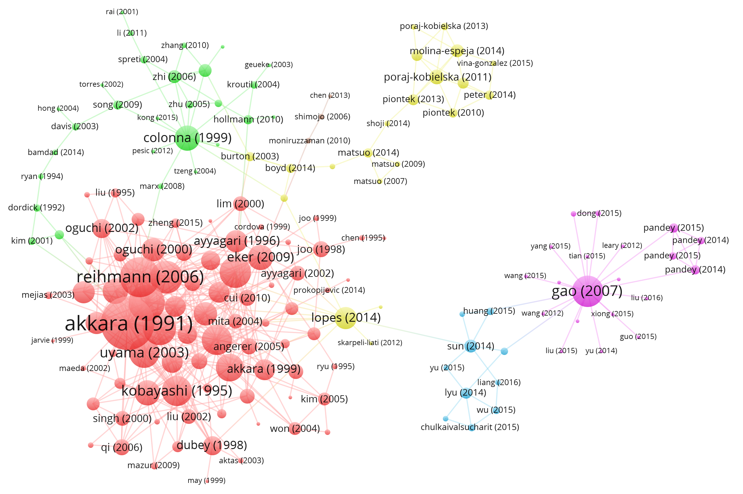
It is easly shown that, among the top 90 authors by degree, there is a big dominant community including most of them. The other communities have got a low number of nodes with respect to the dominant one.
There are also a few connected components (detached from the big one) which form micro-communities.

---

4. Command Line Question (CLQ)

# # Question 1
# echo "Is there any node that acts as an important "'connector'" between the different parts of the graph?"
# grep -o 'target="[0-9]*"' citation_graph.graphml | cut -d'"' -f2 | sort | uniq -c | sort -nr | head -n 1
# # Question 2
# echo "How does the degree of citation vary among the graph nodes?"
# max=$(grep -o 'target="[0-9]*"' citation_graph.graphml | cut -d'"' -f2 | sort | uniq -c | sort -nr | awk '{print "Ranges from " $1}' | head -n 1)
# min=$(grep -o 'target="[0-9]*"' citation_graph.graphml | cut -d'"' -f2 | sort | uniq -c | sort -nr | awk '{print "to " $1}' | tail -n 1)
# echo "Ranges from $max to $min"
# # Question 3
# echo "What is the average length of the shortest path among nodes?"

# # pip install networkx
# python -c'
# import networkx as nx

# # Load the graph from a GraphML file
# G = nx.read_graphml("citation_graph.graphml")
# sum = 0
# # Check if the graph is strongly connected
# if nx.is_strongly_connected(G):
#     average_distance = nx.average_shortest_path_length(G)
#     print(f"Average shortest path length: {average_distance}")
# else:
#     print("Graph is not strongly connected.")

#     # Calculate average shortest path length for each connected component
#     components = list(nx.strongly_connected_components(G))
#     for i, component in enumerate(components, start=1):
#         subgraph = G.subgraph(component)
#         component_average_distance = nx.average_shortest_path_length(subgraph)
#         sum = sum + component_average_distance
#     print(f"Average shortest path length: {sum/i}")
# '

Explaination of what is done in each part

1. Question 1:

• It looks for instances of the goal nodes in a list links or mentions (known by 'target' feature).
• Cuts the node IDs from text using Unix tools like cut.
• Uses uniq -c to count the number of times each node ID appears.
• Sorts the counts in a way that goes down from biggest to smallest using sort -nr.
• Displays the first line, with the largest count done by get head -n 1.
• This gives the node number, seen as a possible linker among various parts of the illustration.

2. Question 2:

• Like Question 1, it measures how often the target nodes show up in a citation graph and lists them.
• Uses awk to arrange the results like "Ranges from X" where X is input.
• It locates the highest and lowest counts.
• Provides information about the differing levels of connections that nodes have.

3. Question 3:

• Checks if a social network is really linked using NetworkX.
• If very connected, it caves and shows the average quickest path length for the whole picture.
• If not well connected, it figures out the average shortest path length for each part of those components that are strongly linked. These parts should be studied one by one separately.
• Shows the average length of shortest paths in total, looking at all parts connected together.

---

5. Algorithmic Questions (AQ)

Part A

1. Implement an algorithm to solve the described mentioned problem.

def skillScore():
    # Line 1 input: (N, M and S)
    N, M, S = input("Enter N, M and S values space separated: ").split(" ")
    N, M, S = int(N), int(M), int(S)

    # Line 2 input: Set of skills (S)
    skillsReq = input("Enter skills space separated: ").split(" ")

    # Line 3 input: Player id, Skill and Skill score

    skillsAndSkillScore = {}
    # skillsAndSkillScore = []

    for i in range(N):
        playerId = int(input())
        for ii in range(S):
            playerSkill, skillScore = input().split()
            if playerSkill in skillsAndSkillScore:
                skillsAndSkillScore[playerSkill].append(int(skillScore))
            else:
                skillsAndSkillScore[playerSkill] = [int(skillScore)]

    teamScore = 0

    # Sort Scores

    for key, _ in skillsAndSkillScore.items():
        skillsAndSkillScore[key] = sorted(skillsAndSkillScore[key], reverse=True)

    print("Sorted scores are: ", skillsAndSkillScore)

    for skill in skillsReq:
        if skill in skillsAndSkillScore:
            if len(skillsAndSkillScore[skill]) <= 0:
                teamScore += 0
            else:
                score = skillsAndSkillScore[skill].pop(0)
                teamScore += score
        else:
            teamScore += 0
        print("Skills and skill score is: ", skillsAndSkillScore)
        print("Team score is: ", teamScore)

    return teamScore

#Inserting input 1
out1 = skillScore()
out1

Sorted scores are:  {'BSK': [98], 'ATH': [52, 14], 'HCK': [95, 82, 9], 'FTB': [90], 'TEN': [85], 'RGB': [46], 'SWM': [59, 34, 16], 'VOL': [32], 'SOC': [41]}
Skills and skill score is:  {'BSK': [98], 'ATH': [52, 14], 'HCK': [95, 82, 9], 'FTB': [90], 'TEN': [85], 'RGB': [46], 'SWM': [34, 16], 'VOL': [32], 'SOC': [41]}
Team score is:  59
Skills and skill score is:  {'BSK': [98], 'ATH': [52, 14], 'HCK': [95, 82, 9], 'FTB': [90], 'TEN': [85], 'RGB': [46], 'SWM': [34, 16], 'VOL': [], 'SOC': [41]}
Team score is:  91
Skills and skill score is:  {'BSK': [98], 'ATH': [14], 'HCK': [95, 82, 9], 'FTB': [90], 'TEN': [85], 'RGB': [46], 'SWM': [34, 16], 'VOL': [], 'SOC': [41]}
Team score is:  143
Skills and skill score is:  {'BSK': [98], 'ATH': [14], 'HCK': [95, 82, 9], 'FTB': [90], 'TEN': [85], 'RGB': [46], 'SWM': [34, 16], 'VOL': [], 'SOC': [41]}
Team score is:  143
Skills and skill score is:  {'BSK': [98], 'ATH': [14], 'HCK': [95, 82, 9], 'FTB': [90], 'TEN': [85], 'RGB': [46], 'SWM': [34, 16], 'VOL': [], 'SOC': [41]}
Team score is:  143
Skills and skill score is:  {'BSK': [], 'ATH': [14], 'HCK': [95, 82, 9], 'FTB': [90], 'TEN': [85], 'RGB': [46], 'SWM': [34, 16], 'VOL': [], 'SOC': [41]}
Team score is:  241
Skills and skill score is:  {'BSK': [], 'ATH': [14], 'HCK': [82, 9], 'FTB': [90], 'TEN': [85], 'RGB': [46], 'SWM': [34, 16], 'VOL': [], 'SOC': [41]}
Team score is:  336
Skills and skill score is:  {'BSK': [], 'ATH': [14], 'HCK': [82, 9], 'FTB': [90], 'TEN': [85], 'RGB': [46], 'SWM': [34, 16], 'VOL': [], 'SOC': [41]}
Team score is:  336
Skills and skill score is:  {'BSK': [], 'ATH': [14], 'HCK': [82, 9], 'FTB': [90], 'TEN': [85], 'RGB': [46], 'SWM': [16], 'VOL': [], 'SOC': [41]}
Team score is:  370
Skills and skill score is:  {'BSK': [], 'ATH': [14], 'HCK': [82, 9], 'FTB': [90], 'TEN': [85], 'RGB': [46], 'SWM': [16], 'VOL': [], 'SOC': [41]}
Team score is:  370

370

#Inserting input 2
out2 = skillScore()
out2

Sorted scores are:  {'BSK': [98, 12], 'HCK': [95, 82, 50, 40, 12, 9], 'ATH': [52, 30, 14], 'VOL': [32, 20, 1], 'SWM': [59, 34, 30, 27, 16, 11], 'FTB': [90, 12], 'RGB': [80, 46, 7], 'TEN': [85, 82], 'SOC': [41]}
Skills and skill score is:  {'BSK': [98, 12], 'HCK': [95, 82, 50, 40, 12, 9], 'ATH': [52, 30, 14], 'VOL': [32, 20, 1], 'SWM': [34, 30, 27, 16, 11], 'FTB': [90, 12], 'RGB': [80, 46, 7], 'TEN': [85, 82], 'SOC': [41]}
Team score is:  59
Skills and skill score is:  {'BSK': [98, 12], 'HCK': [95, 82, 50, 40, 12, 9], 'ATH': [52, 30, 14], 'VOL': [20, 1], 'SWM': [34, 30, 27, 16, 11], 'FTB': [90, 12], 'RGB': [80, 46, 7], 'TEN': [85, 82], 'SOC': [41]}
Team score is:  91
Skills and skill score is:  {'BSK': [98, 12], 'HCK': [95, 82, 50, 40, 12, 9], 'ATH': [30, 14], 'VOL': [20, 1], 'SWM': [34, 30, 27, 16, 11], 'FTB': [90, 12], 'RGB': [80, 46, 7], 'TEN': [85, 82], 'SOC': [41]}
Team score is:  143
Skills and skill score is:  {'BSK': [98, 12], 'HCK': [95, 82, 50, 40, 12, 9], 'ATH': [30, 14], 'VOL': [1], 'SWM': [34, 30, 27, 16, 11], 'FTB': [90, 12], 'RGB': [80, 46, 7], 'TEN': [85, 82], 'SOC': [41]}
Team score is:  163
Skills and skill score is:  {'BSK': [98, 12], 'HCK': [95, 82, 50, 40, 12, 9], 'ATH': [30, 14], 'VOL': [], 'SWM': [34, 30, 27, 16, 11], 'FTB': [90, 12], 'RGB': [80, 46, 7], 'TEN': [85, 82], 'SOC': [41]}
Team score is:  164
Skills and skill score is:  {'BSK': [12], 'HCK': [95, 82, 50, 40, 12, 9], 'ATH': [30, 14], 'VOL': [], 'SWM': [34, 30, 27, 16, 11], 'FTB': [90, 12], 'RGB': [80, 46, 7], 'TEN': [85, 82], 'SOC': [41]}
Team score is:  262
Skills and skill score is:  {'BSK': [12], 'HCK': [82, 50, 40, 12, 9], 'ATH': [30, 14], 'VOL': [], 'SWM': [34, 30, 27, 16, 11], 'FTB': [90, 12], 'RGB': [80, 46, 7], 'TEN': [85, 82], 'SOC': [41]}
Team score is:  357
Skills and skill score is:  {'BSK': [], 'HCK': [82, 50, 40, 12, 9], 'ATH': [30, 14], 'VOL': [], 'SWM': [34, 30, 27, 16, 11], 'FTB': [90, 12], 'RGB': [80, 46, 7], 'TEN': [85, 82], 'SOC': [41]}
Team score is:  369
Skills and skill score is:  {'BSK': [], 'HCK': [82, 50, 40, 12, 9], 'ATH': [30, 14], 'VOL': [], 'SWM': [30, 27, 16, 11], 'FTB': [90, 12], 'RGB': [80, 46, 7], 'TEN': [85, 82], 'SOC': [41]}
Team score is:  403
Skills and skill score is:  {'BSK': [], 'HCK': [82, 50, 40, 12, 9], 'ATH': [30, 14], 'VOL': [], 'SWM': [30, 27, 16, 11], 'FTB': [90, 12], 'RGB': [80, 46, 7], 'TEN': [85, 82], 'SOC': [41]}
Team score is:  403

403

1. Input Collection:

• Takes three space-separated inputs: N is the number of players, M represents skills and S shows how many abilities a team requires.
• The team wants a list of abilities, which should be divided by spaces.

2. Player Skill and Score Storage:

• Begin a list (skillsAndSkillScore) to store player abilities and their related scores.
• It goes through every player and gets their ID with skill-score pairs.
• This info is stored in the dictionary.

3. Sorting Scores:

• Sort the scores for each skill from best to worst.

4. Team Score Calculation:

• Makes a variable (teamScore) equal to zero.
• Repeats the essential skills needed for a group.
• For each skill:
• Checks if the ability is in the player's skills.
• If present:
• Checks if the skill has a score.
• If there is one, it gets the highest mark. It adds that to the team's total and takes it away from a list of scores.
• If they don't have it, the team gets 0 points.
• If you don't have the skill, it won't help your team score points.
• Shows the updated skillsAndSkillScore and current team score.

5. Final Output:

• Prints the final team score.

2. What is the time complexity (the Big O notation) of your solution? Please provide a detailed explanation of how you calculated the time complexity.

O(N * S * log(S)), where N is the number of players and S is the number of skills, is the time complexity. This computation is O(N * S), which is the result of stacked loops that iterate over the players and talents. O(N * S * log(S)) is the total time complexity as a result of the sorting process for every skill inside the loops, which also introduces a factor of log(S). Taking into account the worst-case situation, this notation shows how the execution time increases as the input size increases. Because the sorting step is log-linear, it impacts the algorithm's efficiency and adds to the time complexity dominating factor.

3. Ask ChatGPT or any other LLM chatbot tool to check your code's time complexity (the Big O notation). Compare your answer to theirs. If the two differ, which one is right? (why?)

Analyzing the code step by step, the overall time complexity of the skillScore function can be determined as follows:

Time Complexity of skillScore():

1. Input Processing:

   • Reading N, M, and S: O(1)
   • Reading skillsReq: O(S)
   • Reading player data: O(N * S)

2. Constructing skillsAndSkillScore dictionary:

   • Inserting elements into a dictionary: O(1) for each insertion
   • Insertions are performed for N * S elements
   • Total time complexity: O(N * S)

3. Sorting skillsAndSkillScore dictionary:

   • Sorting a dictionary's values: O(N * S * log(S))

4. Calculating teamScore:

   • For each skill in skillsReq:
     • Checking if skill exists: O(1)
     • Checking if skill score exists: O(1)
     • Checking if skill score is non-empty: O(1)
     • Adding skill score to teamScore: O(1)
   • Iteration over skillsReq: O(S)
   • Total time complexity for skill score calculations: O(S)

Overall Time Complexity:

Summarizing the individual time complexities:

• Input Processing: O(1) + O(S) + O(N * S) = O(N * S)
• skillsAndSkillScore Construction: O(N * S)
• skillsAndSkillScore Sorting: O(N * S * log(S))
• TeamScore Calculation: O(S)

Therefore, the overall time complexity of the skillScore function is O(N * S * log(S)). This means that the function's execution time will grow linearly with the number of players (N) and the number of skills per player (S), and will also logarithmically increase with the number of skills required (S).

4. If your algorithm has exponential time complexity, can you provide a polynomial-time version?

It has polynomial time complexity

5. If S = 1 how does the time complexity of an optimal algorithm to solve this problem change?

⁤O(N), where N is the number of players, is the temporal complexity of the method if S is constant and set to 1. ⁤⁤Since there is only one talent in this case, the sorting process inside the loop that iterates over the skills (S) becomes a constant time operation. ⁤

Part B

1. Prove or disprove that the problem is NP-complete.

To see if the question is NP-complete or not, it should meet both the NP and NP-hard requirements.

For NP:

If a hassle has a verifiable solution in polynomial time, it belongs to the complexity class NP. Verifying that the team has all of the necessary capabilities and that the overall effort to collaborate is stored to a minimum is one manner to affirm an answer for the problem undertaking. This may be completed by engaging in a depth-first search at the graph G in polynomial time. As a result, it is a NP problem.

For NP-Hard:

If an issue may be solved in polynomial time for each different problem within the complexity elegance NP, then it is stated to be NP-hard. We ought to present a polynomial-time discount from every other NP-hard problem to the problem trouble as a way to reveal the NP-hard of the trouble.

The Set Cover trouble is one suitable trouble to remember. One famous NP-complete hassle is the Set Cover hassle, which asserts that:

Determine the smallest subcollection of C that encompasses S given a hard and fast of items S and a group of subsets C of S.

We can construct a graph G on this manner to simplify the Set Cover hassle to the problem trouble:

Every detail in S is matched with a node in G. A clique in G corresponds to each subset in C. The effort needed for the matching crew members to collaborate effectively is the load of an edge connecting two nodes. Next, through determining the minimal spanning tree of G, we are able to decide the smallest subcollection of C that encompasses S.

As a end result, in polynomial time, the problem trouble can be simplified to the Set Cover hassle. This implies that the problem trouble may be solved in polynomial time the use of any technique which can clear up the Set Cover hassle. It follows that since the Set Cover hassle is NP-difficult, so is the problem hassle.

2. Write a heuristic in order to approximate the best solution for this problem.

Randomised Greedy Heuristic Though it adds unpredictability to the selection process, this heuristic is comparable to the greedy heuristic. Rather than choosing the player with the greatest skill score for each required skill, the heuristic chooses a participant at random from the pool of eligible players. This may lessen the possibility of becoming trapped in local optima.

Begin with a team of no members. Add the player with the greatest skill score for any necessary talents who isn't on the squad yet. (greedy method) Until the team has all the information required, repeat step 2 as necessary.

Pros: Less likely to get stuck in local optima Cons: May not find the optimal solution

3. What is the time complexity of your solution ?

O(N * S * log(S)) is the counter's time complexity. Since the heuristic needs to be applied to every player (N), discover the necessary skill that each player has the highest skill score for (S). A priority queue, whose temporal complexity is O(log) over (S)), can be used to achieve this.